Equation Solving

More about Equation Solving

For more about equation solving please refer to another notebook of mine: Intelligence.

There are so many methods and techniques to solve an equation. Here we will review only some of them.

Ordinary Differential Equations

There are many important equations in physics.

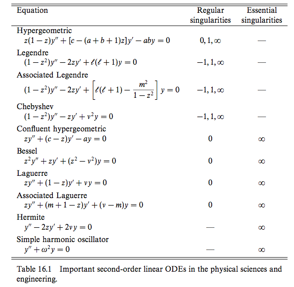
Fig. 10 Taken from Riley’s book.

The are many methods to solve an ODE,

1. Green’s function.
2. Series solution
3. Laplace transform
4. Fourier transform

Green’s Function

Definition of Green’s Function

The idea of Green/s function is very simple. To solve a general solution of equation

(1)\[\frac{d^2}{d x^2} y(x) + y(x) = f(x),\]

where \(f(x)\) is the source and some given boundary conditions. To save ink we define

\[\hat L_x = \frac{d^2}{dx^2} + 1,\]

which takes a function \(y(x)\) to \(f(x)\), i.e.,

(2)\[\hat L_x y(x) = f(x).\]

Now we define the Green’s function to be the solution of equation (2) but replacing the source with delta function \(\delta (x-z)\)

\[\hat L_x G(x,z) = \delta(z-x).\]

Why do we define this function? The solution to equation (1) is given by

\[y(x) = \int G(x,z) f(z) dz.\]

To verify this conclusion we plug it into the LHS of equation (1)

\[\begin{split}& \left(\frac{d^2}{dx^2} +1 \right) \int G(x,z) f(z) dz \\ =& \int \left[ \left(\frac{d^2}{dx^2} +1 \right) G(x,z) \right] f(z) dz \\ =& \int \delta(z-x) f(z) dz \\ =& f(x),\end{split}\]

in which we used one of the properties of Dirac delta distribution

\[\int f(z) \delta(z-x) dz = f(x).\]

Also note that delta function is even, i.e., \(\delta(-x) = \delta(x)\).

So all we need to do to find the solution to a standard second differential equation

\[\left( \frac{d^2}{dx^2} + p(x) \frac{d}{dx} + q(x) \right)y(x) = f(x)\]

is do the following.

1. Find the general form of Green’s function (GF) for operator for operator \(\hat L_x\).

2. Apply boundary condition (BC) to GF. This might be the most tricky part of this method. Any ways, for a BC of the form \(y(a)=0=y(b)\), we can just choose it to vanish at a and b. Otherwise we can move this step to the end when no intuition is coming to our mind.

3. Continuity at \(n-2\) order of derivatives at point \(x=z\), that is

   \[G^{(n-2)}(x,z) \vert_{x<z} = G^{(n-2)} \vert _{x>z} ,\qquad \text{at } x= z.\]

4. Discontinuity of the first order derivative at \(x=z\), i.e.,

   \[G^{(n-1)}(x,z)\vert_{x>z} - G^{(n-1)}(x,z)\vert_{x<z} = 1, \qquad \text{at } x= z.\]

   This condition comes from the fact that the integral of Dirac delta distribution is Heaviside step function.

5. Solve the coefficients to get the GF.

6. The solution to an inhomogeneous ODE \(y(x)=f(x)\) is given immediately by

   \[y(x) = \int G(x,z) f(z) dz.\]

   If we haven’t done step 2 we know would have some unkown coefficients which can be determined by the BC.

How to Find Green’s Function

So we are bound to find Green’s function. Solving a nonhonogeneous equation with delta as source is as easy as solving homogeneous equations.

We do this by demonstrating an example differential equation. The problem we are going to solve is

\[\left(\frac{d^2}{dx^2} + \frac{1}{4}\right) y(x) = f(x),\]

with boundary condition

(3)\[y(0) = y(\pi) = 0.\]

For simplicity we define

\[\hat L_x = \frac{d^2}{dx^2} + \frac{1}{4}.\]

First of all we find the GF associated with

\[\hat L_x G(x,z) = \delta(z-x).\]

We just follow the steps.

• The general solution to

  \[\hat L_x G(x,z) = 0\]

  is given by

  \[\begin{split}G(x,z) = \begin{cases} A_1\cos (x/2) + B_1 \sin(x/2), & \qquad x \leq z, \\ A_2\cos (x/2) + B_2 \sin(x/2), & \qquad x \geq z. \end{cases}\end{split}\]

• Continuity at \(x=z\) for the 0th order derivatives,

  \[G(z_-,z) = G(z_+,z),\]

  which is exactly

  (4)\[A_1\cos(z/2) + B_1 \sin(z/2) = A_2 \cos(z/2) + B_2\sin(z/2).\]

• Discontinuity condition at 1st order derivatives,

  \[\left.\frac{d}{dx} G(x,z) \right\vert_{x=z_+} - \left.\frac{d}{dx} G(x,z) \right\vert_{x=z_-} = 1,\]

  which is

  (5)\[-\frac{A_2}{2}\sin\frac{z}{2} + \frac{B_2}{2} \cos\frac{z}{2} - \left( -\frac{A_1}{2}\sin\frac{z}{2} + \frac{B_1}{2}\cos\frac{z}{2} \right) = 1\]

  Now we combine ((4)) and ((5)) to eliminate two degrees of freedom. For example, we can solve out \(A_1\) and \(B_1\) as a function of all other coefficients. Here we have

  \[\begin{split}B_1 &= \frac{ - 2/\sin(z/2) }{\tan(z/2) + \cot(z/2)} + B_2 , \\ A_1 &= A_2 + B_2(\tan(z/2)-1) + \frac{2}{\sin(z/2) + \cot(z/2)\cos(z/2)}.\end{split}\]

• Write down the form solution using \(y(x) = \int G(x,z) f(z) dz\). Then we still have two unknown free coefficients \(A_2\) and \(B_2\), which in fact is to be determined by the BC equation (3).

Series Solution

A second order ODE,

\[y''(x)+p(x) y'(x) + q(x)y(x)=0\]

Wronskian of this is

\[\begin{split}W(x) = \begin{vmatrix} y_1 & y_2 \\ y_1' & y_2' \end{vmatrix},\end{split}\]

where \(y_1\) and \(y_2\) are linearly independent solutions, i.e., \(c_1 y_1 + c_2 y_2=0\) is only satisfied when \(c_1=c_2=0\). Wronskian is NOT zero if they are linearly independent.

Singularities of an ODE is are defined when \(p(x)\) or \(q(x)\) or both of them have singular points. For example, Legendre equation

\[(1-z^2) y'' - 2 z y' + l(l+1) y = 0\]

has three singular points which are \(z=\pm 1, \infty\) while \(z=0\) is an ordinary point.

Solution at Ordinary Points

Series expansion of the solution can be as simple as

\[y(z) = \sum_{n=0}^{\infty} a_n z^n,\]

which converges in a radius \(R\) where \(R\) is the distance from \(z=0\) to the nearest singular point of our ODE.

Solution at Regular Singular Points

Frobenius series of the solution

\[y(z) = z^\sigma \sum_{n=0}^{\infty} a_n z^n.\]

The next task is to find the indicial equation.

If the roots are not differing by an integer, we just plug the two solutions to \(\sigma\) in and find two solutions independently.

If the roots differ by an integer, on the other side, we can only plug in the larger root and find one solution. As for the second solution, we need some other techniques, such as Wronskian method and derivative method.

Wronskian method requires two expression of Wronskian, which are

\[\begin{split}W(x) = \begin{vmatrix} y_1 & y_2 \\ y_1' & y_2' \end{vmatrix} ,\end{split}\]

and

\[W(z) = C e^{-\int^z p(u) \mathrm du}.\]

From the first expression, we have

\[y_2(z) = y_1(z) \int^z \frac{W(u)}{y_1(u)^2} \mathrm d u.\]

However, we don’t know \(W(z)\) at this point. We should apply the second expression of Wronskian,

\[y_2(z) = y_1(z) \int^z \frac{C e^{-\int^z p(u) \mathrm du}}{y_1(u)^2} \mathrm d u,\]

where the constant \(C\) can be set to 1 as one wish.

TO DO

The derivative method is on my to do list.

Comparing With A General Form

For equation that take the following form,

\[y'' + \frac{1 - 2a}{x} y' + \left( (b c x^{c-1})^2 + \frac{a^2 - p^2 c^2}{x^2} \right) y = 0,\]

where \(y\equiv y(x)\), we can write down the solutions immediately,

\[y(x) = x^a \mathscr {Z}_p (b x^c),\]

in which \(\mathscr {Z}_p\) is the solution to Bessel equation, i.e., is one kind of Bessel function with index \(p\).

A Pendulum With A Uniformly Chaning String Length

As an example, let’s consider the case of length changing pendulum,

\[\frac{d}{dt} \left( m l^2 \dot{\theta}\right) = - m g l \sin\theta \approx = - m g l \theta.\]

Notice that l is a function of time and

\[l = l_0 + v t.\]

Then the equation can be rewritten as

\[\frac{d^2}{dl^2}\theta + \frac{2}{l} \frac{d}{dl} \theta + \frac{g/v^2}{l} \theta = 0.\]

Comparing with the general form, we have one of the possible solutions

\[\begin{split}a & = -1/2, \\ pc & = 1/2, \\ c & = 1/2, \\ p & = 1, \\ b & = 2\sqrt{g}/v.\end{split}\]

This solution should be

\[\begin{split}\theta &= l^a \mathscr{Z}_p(b l^c) \\ & = \frac{1}{\sqrt{l}} J_1(\frac{2\sqrt{g}}{v} \sqrt{l}).\end{split}\]

Airy Equatioin

Time-independent Schrödinger equation with a simple potential,

\[\ddot{\Psi} + \alpha x \Psi = 0.\]

Comparing it with general form, we should set

\[\begin{split}a & = 1/2, \\ \lvert p c \rvert & = 1/2, \\ c & = 3/2, \\ b^2 c^2 & = \alpha^2.\end{split}\]

So the two possible solutions are

\[\begin{split}\Psi_1(x) & = \sqrt{x} \mathscr{Z}_{1/3}(2/3 \alpha x^{3/2}), \\ \Psi_2(x) & = \sqrt{x} \mathscr{Z}_{-1/3}(2/3 \alpha x^{3/2}).\end{split}\]

The general solution is

\[\Psi(x) = a \Psi_1(x) + b \Psi_2(x).\]

Second Order Differential Equations and Gauss’ Equation

Gauss’ equation has the form

\[z(z-1)\frac{d^2}{dz^2} u(z) + \left[(a+b+1)z -c \right] \frac{d}{dz} u(z) + a b u(z) =0,\]

which has a solution of the hypergeometric function form

\[u(z) = {}_2 F_{1}(a,b;c;z).\]

The interesting part about this equation is that its Papperitz symbol is

\[\begin{split}\begin{Bmatrix} 0 & 1 & \infty & \\ 0 & 0 & a & z \\ 1-c & c-a-b & b & \end{Bmatrix} ,\end{split}\]

in which the first three columns are the singularities at points \(0,1,\infty\) while the last column just points out that the argument of this equation is \(z\).

This means, in some sense, the solution to any equation with three singularities can be directly written down by comparing the equation with Gauss’ equation. If you care, the actual steps are changing variables, rewriting the equation into Gauss’ equation form, writing down the solutions.

Integral Equations

Neumann Series AKA WKB

For differential equation, whenever the highest derivative is multiplied by a small parameter, try this. But generally, the formalism is the following.

First of all, we use Hilbert space \(\mathscr L[a,b;w]\) which means the space is defined on \([a,b]\) with a weight \(w\), i.e.,

\[\braket{f}{g} = \int_a^b dx w(x) f(x) g(x).\]

Quantum Mechanics Books

Notice that this is very different from the notation we used in most QM books.

What is the catch? Try to write down \(\braket{x}{u}\). It’s not that different because one can alway go back to the QM notation anyway.

With the help of Hilbert space, one can alway write down the vector form of some operators. Suppose we have an equation

\[\hat L u(x) = f(x),\]

where \(\hat L=\hat I + \hat M\). So the solution is simply

\[\begin{split}u(x) &= {\hat L}^{-1} f(x)\\ &=(\hat I + \hat M)^{-1} f(x) .\end{split}\]

However, it’s not a solution until we find the inverse. A most general approach is the Neumann series method. We require that

\[\| \hat M u \| < \gamma \| u \|,\]

where \(\gamma\in (0,1)\) and should be independent of \(x\).

As long as this is satisfied, the equation can be solved using Neumann series, which is an iteration method with

\[\begin{split}u(x)&=u_0(x)+ \delta u_1(x) + \delta^2 u_2(x) +\cdots \\ u_0(x) & = f(x).\end{split}\]

As an example, we can solve this equation

\[(\hat I + \ket{t}\bra{\lambda}) u(t) = f(t).\]

We define \(\hat M = \ket{t}\bra{\lambda}\) and check the convergence condition for \(\lambda\).

Step one is always checking condition of convergence.

Step two is to write down the series and zeroth order. Then we reach the key point. The iteration relation is

\[u_n(t) + \int_0^1 ds su_{n-1}(s) = 0.\]

One can write down \(u_1\) imediately

\[u_1(t) = -\int_0^1 ds s u_0(s).\]

Keep on going.

Using Dyads in Vector Space

For the same example,

\[\hat L u(x) = f(x),\]

where \(\hat L=\hat I + \hat M\), we can solve it using vector space if operator is linear.

Suppose we have a \(\hat M=\ket{a}\bra{b}\), the equation, in some Hilbert space, is

\[\ket{u} + \ket{a}\braket{b}{u} = \ket{f}.\]

Multiplying through by \(\bra{b}\), we have

\[\braket{b}{u} + \braket{b}{a}\braket{b}{u} = \braket{b}{f},\]

which reduces to a linear equation. We only need to solve out \(\braket{b}{u}\) then plug it back into the original equation.