Useful Math Tricks

Functional Derivative

By definition, [1] functional derivative of a functional \(G[f]\) with respect to \(f\) along the ‘direction’ of \(h\) is

\[\delta G[f][h] = \frac{d}{d\epsilon} G[f+\epsilon h]\vert_{\epsilon=0}.\]

As an example, the functional derivative of \(G[f]=\int dx f^n(x)\) \(\delta G[f][h]\) is

\[\begin{split}\delta G[f][h] &= \frac{d}{d\epsilon} G[f+\epsilon h] \vert_{\epsilon=0} \\ & = \int nf^{n-1}(x) h(x) dx.\end{split}\]

Now the problem appears. We have an unknown function \(h\) which makes sense because we haven’t specify a direction of the derivative yet.

For a physicist, the savior of integral is Dirac delta. So we use delta distribution as the direction in the functional derivative of action which is an integral,

\[\frac{\delta G[f]}{\delta f(y)} = \delta G[f][\delta_y].\]

It can be ambiguous to just write down \(\delta_y\) without an example. Here is the previous example continued,

\[\begin{split}\frac{\delta G[f(y)]}{\delta f(y)} &= \int nf^{n-1}(x) h(x) dx \vert_{h(x)= \delta(x-y)} \\ & = \int nf^{n-1}(x) \delta(x-y) dx \\ & = n f^{n-1}(y) .\end{split}\]

It seems that we can just think of \(f\) as a variable then take the ordinary derivative with respect to it. It is NOT true.

Consider such a functional \(G[f]=\int (f'(x))^2 dx\) where ‘ means the derivative of \(f(x)\).

\[\begin{split}\frac{\delta G[f]}{\delta f} & = -\int dx 2 f''(x) h(x) \vert_{h(x)=\delta(x-y)} \\ & = -2 f''(y) ,\end{split}\]

which is not that straightforward to understand from function derivatives.

[1]	Chapter 15 of Physical Mathematics

Legendre Transformation

Legendre transformation is NOT just some algebra. Given \(f(x)\) as a function of \(x\), which is shown in blue, we could find the distance between a line \(y=px_i\) and the function value \(f(x_i)\).

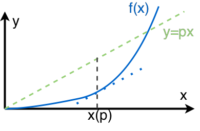
Fig. 2 Meaning of Legendre transformation

However, as we didn’t fix \(x\), this means that the distance

\[F(p,x) = p x - f(x)\]

varies according to \(x\). This is a transformation that maps a function \(f(x)\) to some other function \(F(p,x)\) which depends on the parameter \(p\). A more pedagogical way of writing this is

\[px = F(x,p) + f(x).\]

To have a Legendre transformation, let’s choose a relation between \(x\) and \(p\). One choice is to make sure we have a maximum distance given \(p\), which means the \(x\) we choose is the point that makes the slope of \(f(x)\) the same as the line \(y=px\). In the language of math, the condition we require is

\[0 = \frac{\partial F(p,x)}{\partial x} \equiv f'(x) - p,\]

which indeed shows that the slope of function and slope of the straight line match eath other at the specified point. Thus we have a relation between \(x\) and \(p\).

Substitute \(x(p)\) back into \(F(p,x)\), we will get the Legendre transformation \(F(p,x(p))\) of \(f(x)\).

Back to the math we learned in undergrad study. A Legendre transformation transforms a function of \(x\) to another function with variable \(\frac{f(x)}{x}\). Using \(f(x)\) and its Legendre transformation \(F(p = p x - f(x(p))\) as an example, we can show that the slope of \(F(p)\) is \(x\),

\[\frac{d F(p)}{d p} = x,\]

which is intriging because the slope of \(f(x)\) is \(p\) in our requirement. We removed the dependence of \(x\) in \(F(p)\) because we have this extra constrain.

Let’s Move to Another Level

We require the function \(f(x)\) is convex (second order derivative is not negative ). This is required because otherwise we would NOT have a one on one mapping of \(x\) and \(p\).

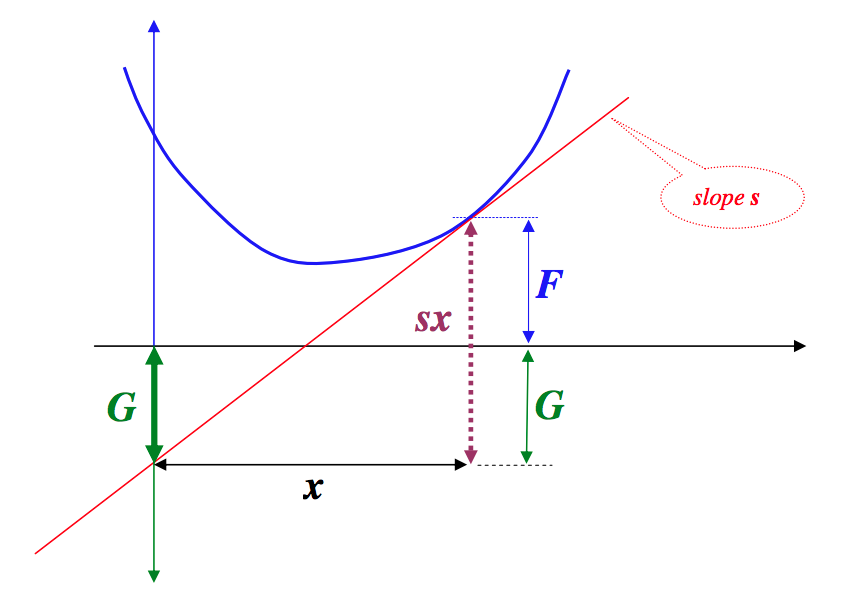
Fig. 3 This graph shows the Legendre transformation and triangles in which G is actually the F we used before and F in the graph corresponds to f.

One imediately notices the symmety of Legendre transformation on interchanging of F and f.

This graph is taken from this paper Making Sense of the Legendre Transform .

This is the triangle that represents the Legendre transformation.

If we have a slope that vanishes, which means \(f(x)\) is at minimium, then we have the relation

Vector Analysis

The ultimate trick is to use component form.

\[\begin{split}&\vec a \times (\vec b \times \vec c) \\ = & \hat e_i \epsilon_{ijk} a_j (\epsilon_{kmn} b_m c_n ) \\ = & \hat e_i \epsilon_{kij}\epsilon_{kmn} a_j b_m c_n \\ = & \hat e_i ( \delta_{im}\delta_{jn} - \delta_{in}\delta_{jm} )a_j b_m c_n \\ = & \hat e_i \delta_{im}\delta_{jn} a_j b_m c_n - \hat e_i \delta_{in}\delta_{jm} a_j b_m c_n \\ = & \hat e_i a_j b_i c_j - \hat e_i a_j b_j c_i \\ = & \vec b (\vec a\cdot \vec c) - \vec c (\vec a \cdot \vec b) .\end{split}\]

One should be able to find the component forms of gradient \(\vec \nabla \cdot\), divergence \(\vec \nabla \times\), Laplace operator, in spherical coordinates, cylindrical coordinates and cartisian coordinates.

Refs & Notes