Electrostatics and Magnetostatics

Electric Field

The electric potential energy of a point charge in an electric field is given by

\[U = q \phi.\]

In the case of fixed point charge \(Q\) field, the amount electric energy of test charge \(q\) is

\[U_q = q\frac{Q}{r}.\]

Suppose we have N point charges places randomly in the space, the total electric energy of the system can be calculated through the a superposition of the electric potential.

\[\begin{split}U &= q_1\sum_{i=1}^N \frac{q_i}{\lvert \vec {x_i} - \vec x \rvert} + \cdots \\ & = \frac{1}{2}\left( \sum_{i\neq j} \frac{q_i q_j}{\lvert \vec {x_i} - \vec {x_j}} \right),\end{split}\]

in which the half is due to the double counting of the interactions.

Energy Density

The next question we are going to consider is the electric potential energy of a bulk charged object.

\[U = \frac{1}{2} \int \rho(\vec x)\phi(\vec x) d^3 x,\]

where

\[\phi(\vec x) = \int \frac{\rho(\vec x')}{ \lvert \vec x - \vec x' \rvert } d^3x'.\]

Derivation of Electric Energy of Charged Object

Construct the system by adding small amount of charge to it from zero charge distribution.

Charge distribution \(\rho(\vec x)\) can be changed linearly \(\lambda \rho(\vec x')\) where \(\lambda\) is a scalar number.

The energy change due to adding charge to the system to change the charge distribution linearly \(\delta \lambda\). Energy change is

\[\delta U = \int \delta \lambda \phi(\vec x) d^3 x.\]

where

\[\phi(\vec x) = \int d^3x' \frac{\lambda \rho(\vec x')}{\lvert \vec x - \vec x' \rvert }.\]

Integrate from 0 to 1 will give us the total energy for an object with charge distribution \(\rho(\vec x)\).

It is obvious that the \(1/2\) comes from the linear dependence of \(\lambda \rho(\vec x)\).

Now we have the expression for energy of electric field, it is straightforward to find the energy density.

1. To calculate that, we need to put together two parts of energy, i.e., E-field outside of the conductor and the surface electric potential energy of the conductor.
2. Then apple the divergence theorem, counting the infinite surface and also all the surfaces of the conductor.
3. Notice the surface integral of the potential energy on the conductor surface is exactly the negative of the surface energy density we put in to the expression in the first step.
4. The surface integral at infinity surface is zero.
5. The only term left is \(-\frac{1}{8\pi}\int d^3x E_i \partial_i \phi=\frac{1}{8\pi}\int d^3x E_i E_i\).

Electric Forces

Alright, move on to the concept of force in E&M. Coloumb force is

\[F_i = \int \rho(\vec x') E_i(\vec x') d^3x'.\]

Maxwell’s equations tells that

\[\rho(\vec x') = \frac{1}{4\pi} \nabla' \cdot \vec E(\vec x').\]

So force can be rewritten as

\[\begin{split}F_i &= \int d^3x' \frac{1}{4\pi} (\partial_j E_j(\vec x') ) E_i(\vec x') \\ & = \frac{1}{4\pi}\int d^3x' ( \partial_j(E_j E_i) - E_j \partial_j E_i )\end{split}\]

Now notice that \(\partial_i(E_j E_j)=2E_j\partial_iE_j\) and \(\partial_i E_j = \partial_j E_i\).

Proof

\[\begin{split}\nabla\times \vec E & = \begin{vmatrix} \hat i & \hat j & \hat k \\ \partial_i & \partial_j & \partial_k \\ E_i & E_j & E_k \end{vmatrix} \\ & = \hat i \epsilon_{ijk} \partial_j E_k.\end{split}\]

So \(\nabla\times \vec E = 0\) means \(\partial_i E_j - \partial_J E_i = 0\).

Force becomes

\[\begin{split}F_i &= \frac{1}{4\pi}\int d^3x' ( \partial_j(E_j E_i) - E_j \partial_j E_i ) \\ & = \frac{1}{4\pi}\int d^3x' ( \partial_j(E_j E_i) - \frac{1}{2}\partial_i (E_jE_j) ) \\ & = \frac{1}{4\pi}\int d^3x' \partial_j ( (E_j E_i) - \frac{1}{2} E^2 ) \\ & = \frac{1}{4\pi}\int d^3x' \partial_j ( (E_i E_j) - \frac{1}{2}\delta_{ij} E_i E_j ) \\ & = \frac{1}{4\pi}\int d^3x' \partial_j ( (1 - \frac{1}{2}\delta_{ij}) E_i E_j ) \\ & = \frac{1}{4\pi}\int dS_{j} (1 - \frac{1}{2}\delta_{ij}) E_i E_j \\\end{split}\]

Recall that force is momentum per unit time. What is inside the integral means some force density or momentum flow density per unit time, for some reason we use the definition

\[T_{ij} = (1 - \frac{1}{2}\delta_{ij}) E_i E_j,\]

which is symmetric under the exchange of i and j.

Stress Tensor in General Relativity or Fluid Dynamics

Electromagnetic energy momentum tensor using Gaussian units and +2 signature is

\[T^{\mu\nu} = c^2 \left( F^{\mu\alpha} F^{\nu}_{\phantom{\mu}\alpha} - \frac{1}{4}\eta^{\mu\nu} F_{\alpha\beta}F^{\alpha\beta} \right),\]

where \(\mathbf F = \mathbf d \mathbf A \Rightarrow F_{\mu\nu} = \partial_\mu A_\nu - \partial_\nu A_\mu\).

\[\begin{split}F^{\mu\nu} \vert_{\text{matrix form}} = \begin{pmatrix} 0 & - E_x/c & - E_y/c & - E_z/c \\ E_x/c & 0 & -B_z & B_y \\ E_y/c & B_z & 0 & -B_x \\ E_z/c & -B_y & B_x & 0 \end{pmatrix}.\end{split}\]

To change the index to \(F^\mu_{\phantom{\mu}\nu}\) we just use the Minkowski metric which just put plus and minus signs on the components,

\[\begin{split}F^{\mu}_{\phantom{\mu}\nu} \vert_{\text{matrix form}} = \begin{pmatrix} 0 & - E_x/c & - E_y/c & - E_z/c \\ -E_x/c & 0 & -B_z & B_y \\ -E_y/c & B_z & 0 & -B_x \\ -E_z/c & -B_y & B_x & 0 \end{pmatrix}.\end{split}\]

Why is this the case? This is because of the Lorentz group requires it. Generators of \(L_+^\uparrow\) which means the orthochronous patch combine together with the infinitesimal change to form the tiny change in Lie algebra, that is to form \(\omega\) in \(L = I +\omega\)

\[\omega = \vec\theta\cdot \vec R + \vec \lambda \cdot \vec B,\]

where the six matrices are basically the generators to construct the Lorentz group.

Energy momentum tensor can be decomposed using the generators,

\[F^{\mu}_{\phantom{\mu}\nu} \vert_{\text{matrix form}} = - E_i B_i + B_i R_i,\]

where we are using the Einstein summation rule.

For more information about this please read arXiv:physics/0005084 .

Force on Capacitor

Suppose we have a capacitor with two parallel round plates of radius \(R\) and separation \(d\). The top plate has charge \(Q\) and bottom plate has charge \(-Q\). Now ask the question, what is the force on the top plate?

Is its magnitude \(F=QE\) because of the fact that the charge \(Q\) is in a electric field \(\vec E\)? NO.

We can calculate the force using several methods like

1. principle of virtual work,
2. stress tensor.

However the result shows that the magnitude of force is only \(F=\frac{1}{2} Q E\), half of the expectation we had at first.

The intuition is that electric field only exists on one side of the plate while \(F=qE\) describes the force of a charged particle emerged in the electric field. Once one knows this, the half comes from the fact that stress only applies on one side of the top plate.

Multipole Expansion

For a charge object with charge distribution \(\rho(\vec x)\), the electic potential is

\[\phi(\vec x) = \int \rho(\vec x')\frac{1}{\lvert \vec x - \vec x' \rvert} d^3 x' .\]

For any general distribution, we can always have \(\frac{1}{\lvert \vec x - \vec x' \rvert}\) expanded and define differential multipoles.

Monopole and Dipole

Before we go into this expansion, a review of the idea of monopole and dipole is very useful.

Monopole is the case of spherical symmetric distribution of electric potential.

\[\rho_0(\vec x) = \frac{Q}{r} = \frac{1}{r} \int d^3x' \rho(\vec x') = \int d^3x' \frac{\rho(\vec x')}{\lvert \vec x \rvert} .\]

Dipole, using the simplest model, is a system of two charged particles with \(\pm Q\) and directed from negative charge to positive charge.

Fig. 14 Electric dipole from wikipedia .

In the language of math, \(\vec q=Q\vec d\). The electric potential is the superposition of the two charges.

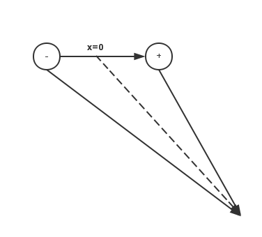
Fig. 15 The dashed line is the position vector \(\vec x\).

\[\begin{split}\phi(\vec x) &= \frac{-Q}{\lvert \vec x -(-\vec d/2) \rvert} + \frac{Q}{\lvert \vec x - \vec d/2 \rvert} \\ &= \int d^3x' \frac{-Q\delta(\vec x' + \vec d/2) + Q \delta(\vec x' -\vec d/2) }{\lvert \vec x - \vec x' \rvert} ??\end{split}\]

I need some time to make clear of different methods.

Dipole comes from the expansion at \(\vec x \gg \vec x'\),

\[\frac{1}{\lvert \vec x - \vec x' \rvert} = \frac{1}{r} + \vec x' \cdot \vec x \frac{1}{r^3} \cdots\]

thus the dipole part is actually

\[\phi_1(\vec x) = \frac{1}{r^3}\vec x \cdot d^3x' \vec x' \rho(\vec x').\]

Multipole

A nth multipole has the dimnsion of \(\frac{[Q]}{[r]} \left(\frac{d}{r}\right)^2\).

In most of the cases, we have a very small dipole compared to the distance at where the field is measured. So we could take the limit that the dipole is point like. The actually meaning of a point dipole is that the dipole is a constant viewed from very far away.

\[\begin{split}\rho(\vec x) &= -q\delta(\vec x + \vec d/2) + q\delta(\vec x -\vec d/2) \\ & \approx -q \nabla\cdot \delta(\vec x) .\end{split}\]

The next question to be answered is the electric field generated by this point dipole.

\[\begin{split}\vec E &= -\nabla \frac{\vec p\cdot \vec x}{r^3} \\ & = \frac{3(\vec p\cdot \vec x)\vec x - \vec p r^2}{r^5} \\ & = \frac{3(\vec p\cdot \vec x)\vec x}{r^5} - \frac{\vec p}{r^3},\end{split}\]

which is only true for \(\vec x \neq 0\).

Force feels by a dipole is

\[\vec F = \nabla(\vec p(\vec x) \cdot \vec E(\vec x) ).\]

Torque can also be calculated

\[\vec \tau = \vec p \times \vec E + \vec x \times \vec F.\]

Force and Torque of Dipole

Force can be calculated using principle of virtual work. \(-\vec p \cdot \vec E\) is the energy which can be explained using simple two charge model.

Torque has two parts, one with a precession-like term which is called spin torque while another one is a orbital torque since it tries to align the dipole with the field lines.

Dielectric Material

In the presence of dielectric material, a new set of quantities will be introduced.

Polarization

Why do we introduce this polarization \(\vec P\)? To make the picture and the math easier to understand, in some sense.

Imagine dielectric material in electric field. Since the material is dielectric, the external electric field induces additional electric field.

We use subscript P for quantities that is induced.

For a neutral object, one conservation law is

\[\int \rho_P(\vec x') d^3x' + \oint \sigma_P \hat n \cdot \vec{dS} = 0,\]

where \(\rho_P\) is the charge volume density distribution inside the object while \(\sigma_P\) is the surface charge density. We need the surface charge because charge will be induced on the surface.

Maxwell’s equations are very beautiful, so we definitely want to preserve Gauss’ law. Thus we define

\[\begin{split}\rho_P(\vec x) &= - \nabla \cdot \vec P_P(\vec x) \\ \sigma_P(\vec x) &= \vec P(\vec x) \cdot \hat n(\vec x).\end{split}\]

Polarization and Electric Field

So what is the relation of \(\vec P\) and \(\vec E\)? This is not trivial. The physics here is the electric field (vector), space distribution, polarization (vector).

\[P_i = ? E_j\]

How many ranks do we need to describe a spatially distribution in Euler space? Two maximum. So

\[P_i = \chi_{ij}E_j .\]

However, the tensor \(\chi_{ij}\) can be a function of \(E_j\) and even \(P_i\).

For isotropic material, we would have no direction dependence of the spatial distribution

\[P_i = \chi E_i .\]

This is because no shear stress is possible thus :math:`P_i` doesn’t depend on E field on other directions.

\(\chi\) can still be a function of \(E_i\) though. Now we require that this material is linear, which means \(\chi\) is independent of \(E_i\).

With the requirement of isotropic and linear, we have a simple relation,

\[P_i = \chi_e E_i,\]

where, for some reason, \(\chi_e\) is called electric suscptibility.

Why is this isotropic and linear approximation useful?

Think about the microscopic structure of material.

Electric Potential

The potential should be related dipole since this is dielectric material. (<- This is a joke.) Anyway, it is related to dipole.

The electric potential is composed of two parts, one produced by the volume charge density and another produced by the surface charge density.

\[\begin{split}\phi_P(\vec x) & =\int d^3x' \frac{\rho(\vec x')}{\lvert\vec x - vec x' \rvert} + \oint \vec{dS'}\cdot \frac{\sigma_P\hat n'}{\lvert \vec x -\vec x'\rvert} \\ & = \int d^3 x' \frac{-\nabla' \cdot \vec P(\vec x')}{\vert\vec x - vec x' \vert} + \oint \vec{dS'} \cdot \frac{\vec P(\vec x')}{\vert\vec x - vec x' \vert} \\ & = \int d^3 x' \frac{-\nabla' \cdot \vec P(\vec x')}{\vert\vec x - vec x' \vert} + \int d^3x' \nabla' \cdot \frac{\vec P(\vec x')}{\vert\vec x - vec x' \vert} \\ & = \int d^3 x' \left( \vec P(\vec x') \cdot \nabla'\cdot \frac{1}{\vert\vec x - vec x' \vert} \right) \\ & = \int d^3 x' \frac{\vec P(\vec x') \cdot (\vec x - \vec x')}{\vert\vec x - vec x' \vert^3} .\end{split}\]

Recall that the electric potential by a dipole is

\[\phi_d = \frac{\vec p\cdot \vec x}{r^3}.\]

The electrical potential generated by induced charge distribution in dielectric material is a integral of a lot dipole electric potential fields. This can be seen by the following approximation in \(x\) direction,

\[(x - x') = x (1 - \frac{x'}{x}) \approx x,\]

then

\[\phi_P(\vec x) \approx \int d^3x' \frac{\vec P(\vec x') \cdot \vec x}{ {\vec x}^3 }.\]

At this point we only considered the induced field.

Total Field

Gauss’ law tells us the field about the total charge, both the original and the induced, and the total field, whatever generated it.

\[\nabla\cdot \vec E = 4\pi (\rho + \rho_P),\]

where \(\rho\) means the free charge.

As we have introduced

\[\rho_P = -\nabla\cdot \vec P,\]

\[\nabla\cdot \vec E = 4\pi (\rho -\nabla\cdot \vec P) .\]

Combine terms

\[\nabla \cdot (\vec E + 4\pi \vec P) = 4\pi \rho.\]

The point is we don’t want to mess with \(\vec P\), so we define a displancement vector

\[\vec D = \vec E + 4\pi \vec P,\]

so that the Gauss’ law only involve with free charge \(\rho\) and the displacement vector,

\[\nabla\cdot \vec D = 4\pi \rho.\]

For isotropic and linear material, we already know \(\vec P = \chi_e \vec E\),

\[\vec D = \vec E + 4\pi \chi \vec E = (1 + 4\pi \chi_e) \vec E,\]

then we define

\[\epsilon = 1 + 4\pi \chi_e,\]

which is the permittivity by definition.

Energy and Stress

Just as a reference,

\[\delta U = \frac{1}{4\pi} \int \vec E \cdot \delta \vec D d^3 x' = \frac{1}{4\pi} \int \frac{1}{2\epsilon}\delta E^2 d^3 x',\]

which indicates that the energy density is

\[u = \frac{1}{8\pi} \vec E\cdot \vec D.\]

Stress tensor \(T_{ij}\) which appears in the formula of force \(\vec F = \int \vec{dS} \cdot \overleftrightarrow{T}\) is

\[T_{ij} = \frac{1}{4\pi} \left( D_i E_j - \frac{1}{2} D_k E_k \delta_{ij} \right).\]

Magnetic Field

Lorentz force is

\[\vec F = q \vec E + q \frac{\vec v}{c}\times \vec B .\]

Ampere‘s Law

Force between two charged wire is given by

\[\vec F = \frac{1}{c^2} \int \int \frac{I_1 \vec{dx} \times ( I_2\vec{dx'} \times (\vec x - \vec x') ) }{\vert \vec x - \vec x'\vert^3}\]

Force on A Charged in Electric Field

Force on a charge in a electric field generated by \(\rho(\vec x)\) is

\[\vec F = q \vec E = q \int d^3x' \frac{\rho(\vec x') (\vec x - \vec x') }{\vert \vec x - \vec x' \vert^3}.\]

Charge Conservation in Magnetostatistics

Conservation of charge means

\[\frac{\partial \rho}{\partial t} + \nabla \cdot \vec j = 0,\]

we require the source of current density 0 which means

\[\frac{\partial \rho}{\partial t} = \nabla\cdot \vec j = 0.\]

The question is how can the electric current feels each other? By intermediate field we say.

Biot-Savart Law

The magnetic field generated by electric current is given by Biot-Savart law.

\[\vec B = \frac{1}{c} \int d^3x' \frac{ vec j(\vec x') \times (\vec x - \vec x') }{\vert \vec x - \vec x' \vert ^3}\]

Starting from magnetic field we could find the force,

\[\vec F = \frac{1}{c}\int d^3x' \vec j(\vec x) \times \vec B (\vec x).\]

Force of Charge Distribution in Electric Field

vec F = int d^3x’ frac{rho(vec x’)} vec E(vec x’) .

Divergence and Curl of Magnetic Field

Using the formula of magnetic field generated by current,

\[\begin{split}\nabla \cdot B &= \frac{1}{c} \nabla\cdot \int d^3x' \vec j(\vec x') \times \frac{\vec x - \vec x'}{\vert \vec x -\vec x' \vert^3} \\ & = \frac{1}{c} \partial_i \int \epsilon_{ikl} j_k(\vec x') \frac{x_l -x_l'}{\vert \vec x - \vec x' \vert^3} d^3x' \\ & = \frac{1}{c} \int j_k \epsilon_{kli} \partial_i \partial_l \frac{1}{\vert \vec x- \vec x' \vert} d^3 x' \\ & = 0\end{split}\]

The last line is true since

\[\begin{split}&j_k \epsilon_{kli} \partial_i \partial_l \frac{1}{\vert \vec x- \vec x'\vert } \\ & = \vec j \cdot (\nabla \times \nabla \frac{1}{\vert \vec x- \vec x'\vert } )\\ & = 0\end{split}\]

The curl on the other hand is not zero.

\[\nabla\times \vec B = \frac{4\pi}{c} \vec j .\]

Apply a loop integral,

\[\oint \vec{dx} \cdot \vec B = \frac{4\pi}{c} I.\]

Vector Potential

For a electric field, we have a scalar potential,

\[\vec E = - \nabla \phi,\]

since electrostatics is curl free,

\[\nabla \times \vec E = - \nabla \times \nabla \phi =0 .\]

Magnetostatics, on the other hand, is divergence free. Thus we expect

\[\vec B = \nabla\times \vec A.\]

Not surprisingly, we have

\[\vec A' = \vec A + \nabla \chi,\]

is also a valid vector potential for \(\vec B\).

Gauges

Coulomb gauge is

\[\nabla \cdot \vec A = 0.\]

Example of Gauge Freedom

To have a magnetic field \(\vec B = B_0 \hat {e_z}\), we could use different vector potentials,

\[\begin{split}\vec A_1 &= B_0 x \hat{e_y}, \\ \vec A_2 & = - B_0 y\hat{e_x}, \\ \vec A_3 & = \frac{\vec A_1 + \vec A_2}{2}.\end{split}\]

This is the gauge freedom of the magnetic field.

Refs & Notes