Curved Spacetime

Christoffel Symbol

By definition, Christoffel symbol is defined through

\[\frac{\partial}{\partial x^\beta} \mathbf e_\alpha = \Gamma^\mu_{\alpha\beta} \mathbf e_\mu.\]

So what it means geometrically, is the small change in the basis vector \(\mathbf e_\alpha\) when we change the coordinate \(x^\beta\), then project it on to the basis vector \(\mathbf e_\mu\).

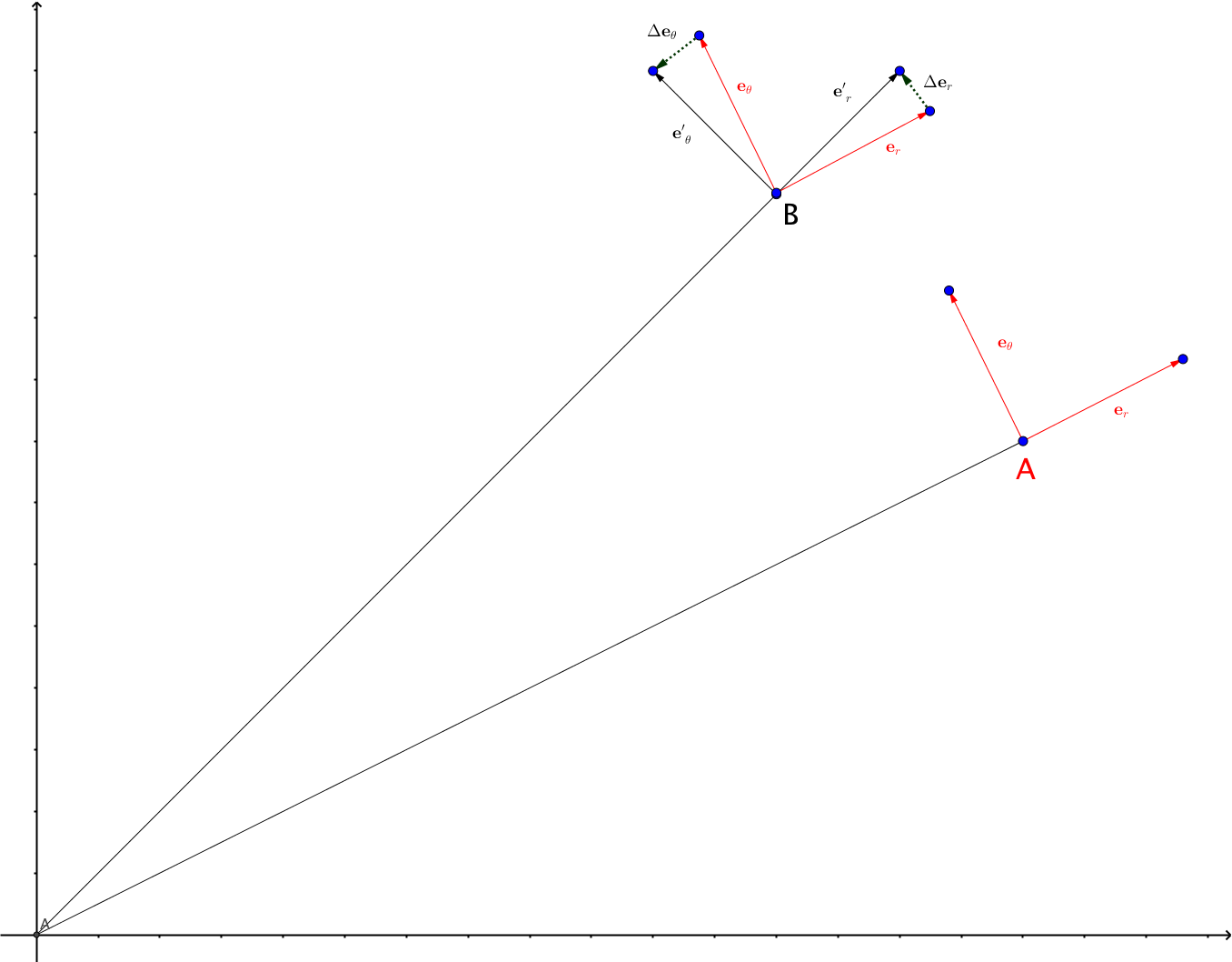
Fig. 24 Christoffel symbol tells us the change in the basis when we move around a little bit. This is an example of polar coordinate system.

In polar coordinate system, the basis change when we move from one point to another. At point A, the basis vectors are shown as red while the basis vectors at point B are shown as black. The two sets of basis vectors are different when we look at it. The change of the vectors are described by \(\frac{\partial}{\partial x^\beta} \mathbf e_\alpha\), which are shown as dotted vectors \(\Delta \mathbf e_\theta\) and \(\Delta \mathbf e_r\). These are calculatable fairly easily. Then we project these vectors onto the basis to get the components of Christoffel symbol.

Curvature

1. Usually curvature is about calculating distances locally. If the distances are the same as flat space, it dosn’t have intrinsic curvature, for example, a cylinder. However, a cylinder has extrinsic curvature because it is curved by our common sense.
2. We can use a plane that is tangent to a point on a surface to determine wether it has intrinsic curvature. Move the plane parallelly up and down from this initial point. If the interceptions are straight lines, we do not expect intrinsic curvature. If the interceptions are conic sections, we expect it to has intrinsic curvature.
3. This indicates that we need to compare two different directions to really know wether the curvature is intrinsic.
4. In fact Gaussian curvature can be calculated using two principal curvatures in different directions.
5. Gauss map is the way that Gauss defined to calculate the Gaussian curvature. It maps an area from the surface onto a unit sphere.

Parallel Transport

1. On a sphere, transporting a vector leads to strange results.
2. All the tangent vectors at different parameters of the curve specifies the curve itself.
3. Parallel transport generally require the vector to be parallel locally with each infinitesimal move.
4. Parallel transport can also be explained as the components along of the vector that we are transporting doesn’t change.
5. Mathematically, \(\frac{d}{d\lambda}V^\alpha=0\) at a locally inertial frame.
6. It can be written as covariant derivative thus genralized to all frames. \(\frac{d}{d\lambda}V^\alpha = U^\beta V^\alpha_{,\beta}=U^\beta V^\alpha_{;\beta}=0\).
7. Another notation is \(\nabla_{\mathbf V}\mathbf V=0\).

Geodesics

1. Euclid’s straight lines indicates that the direction is the key to define straight lines.

2. They are lines that is formed by parallel transporting their own tagent vectors.

3. Generalize to curved spacetime. \(\nabla_{\mathbf V}\mathbf V=0\). It is dubbed as the geodesic.

4. We can find all the coordinates of the geodesic by using the definition of tagent vectors.

   \[\frac{d}{d\lambda}\left( \frac{dx^\alpha}{d\lambda} \right) + \Gamma^\alpha_{\mu\alpha} \frac{dx^\mu}{d\lambda} \frac{dx^\alpha}{d\lambda} =0.\]

4. Second order DE: given initial point and the inital tagent vector we can solve it.
5. \(\lambda\) is the affine parameter.
6. A linear transformation of the affine parameter is usually still a affine parameter.
7. Solve the equation for inertial frame and draw the lines. We’ll see it really describes a straight line.

Geodesics are the lines that describe the extemal length between two points. To prove that we need to write down the length between two lines. From \(ds^2 = g_{\alpha\beta}dx^\alpha dx^\beta\),

\[l = \int_{\lambda_1}^{\lambda^2} \sqrt{ g_{\alpha\beta} \frac{dx^\alpha}{d\lambda}\frac{dx^\beta}{d\lambda} } d\lambda.\]

Then we do the variation of length. Before we actually do it, it’s good to think about what the plan is. We will derive a equation, aka, the geodesic equation, for all coordinates, which indicates that we need to derive a Euler-Lagrange like equation. So we will finally write down the variation of length in a form

\[\delta l \sim \int_{\lambda_1}^{\lambda_2} (\cdots)_\alpha \delta x^\alpha d\lambda,\]

which should be 0 if we require it to be the extemal length.

Mathematics to Prove Geodesic is the Extemal Line

In principle, we could define a Lagrangian and use Euler-Lagrange equation. But here I will demonstrate it using the variation principle.

\[\begin{split}\delta l &= \frac{1}{2} \int_{\lambda_1}^{\lambda_2} \left( g_{\alpha\beta} \frac{d x^\alpha}{d\lambda} \frac{d x^\beta}{d\lambda} \right)^{-1/2} \left( (\delta g_{\alpha\beta}) \frac{d x^\alpha}{d\lambda} \frac{d x^\beta}{d\lambda} + g_{\alpha\beta} \left(\delta\frac{d x^\alpha}{d\lambda} \right) \frac{d x^\beta}{d\lambda} + g_{\alpha\beta} \frac{d x^\alpha}{d\lambda} \left( \delta \frac{d x^\beta}{d\lambda} \right) \right) d\lambda\\ & = \frac{1}{2} \int_{\lambda_1}^{\lambda_2} \left( g_{\alpha\beta} \frac{d x^\alpha}{d\lambda} \frac{d x^\beta}{d\lambda} \right)^{-1/2} \left( (\delta g_{\alpha\beta}) \frac{d x^\alpha}{d\lambda} \frac{d x^\beta}{d\lambda} + 2 g_{\alpha\beta} \left(\delta\frac{d x^\alpha}{d\lambda} \right) \frac{d x^\beta}{d\lambda} \right) d\lambda,\end{split}\]

where we used the symmetry in :math:``{}_{alphabeta} in the last step.

So we need to calculate \(\delta g_{\alpha\beta}\)

\[\begin{split}\delta g_{\alpha\beta} &= \frac{ g_{\alpha\beta}(x^\mu + \delta x^\mu) - g_{\alpha\beta}(x^\mu) }{\delta x^\mu} \delta x^\mu = g_{\alpha\beta,\mu} \delta x^\mu \\ \delta \frac{d x^\alpha}{d\lambda} & = \frac{d \delta x^\alpha}{d\lambda}.\end{split}\]

Plug this in and sort out the total derivatives then we have an expression

\[\delta l = \frac{1}{2}\int_{\lambda_1}^{\lambda_2} S \left( g_{\alpha\beta,\mu} \frac{dx^\alpha}{d\lambda} \frac{dx^\beta}{d\lambda} - 2 \frac{d}{d\lambda}\left(g_{\alpha\mu} \frac{dx^\alpha}{d\lambda} \right) \right) ,\]

where we defined

\[S = \left( g_{\alpha\beta} \frac{d x^\alpha}{d\lambda} \frac{d x^\beta}{d\lambda} \right)^{-1/2}\]

which is a constant since it simply measures the scaling of parameters and length.

Then we use the symmetries in metric and get the Euler-Lagrangian equation which is basically the geodesic equation.

1. The longest length between two points is the time-like geodesic.
2. The time-like geodesic is not necessarily the longest line between two points.
3. We can not find shortest time-like lines between two points.

References and Notes

1. Bernard F. Schutz, A first course in general relativity. Chapter 6.