Basics of Special Relativity

The Postulates, Spacetime Diagram, and Metric

Special relativity was developed out of two postulates [Schutz2009]

1. Princple of relativity (Galileo),
2. Universality of speed of light (Einstein).

Using these two postulates, where the first key definition is interval of events squared

\[\Delta s^2,\]

we can derive basically all the relations we need. Some other intuitions will also be applied to the derivations.

Using a spacetime diagram, we can prove that this is invariant under transformation of frames [Schutz2009].

Hyperbolic Space

If anyone realizes that spacetime is in fact hyperbolic space by looking at the expression of intervals \(\Delta s^2\), the transformation is determined.

As we know the invariant quantity of the physical laws, the transformation of vectors can be found out of it, which is basically a rotation in hyperbolic space.

Metric Conventions

The metric in Eq. (9) is ‘derived’ from the interval.

To write it down, there are different convention. We choose the signature \(+2\) metric in special relativity

\[\begin{split}\eta_{\mu\nu}=\begin{pmatrix} -1 & 0 & 0 & 0\\ 0 & 1 & 0 & 0\\ 0 & 0 & 1 & 0\\ 0 & 0 & 0 & 1\\ \end{pmatrix}.\end{split}\]

In most cases, we use natural unit \(c=1\).

d’Alembert operator

d’Alembert operator, or wave operator, is the Lapace operator in Minkowski space. [1]

\[\Box \equiv \partial _ \mu\partial^\nu = \eta _{\mu\nu}\partial^\mu \partial^\nu\]

In the usual {t,x,y,z} natural orthonormal basis,

\[\begin{split}\Box & = -\partial_t^2+\partial_x^2+\partial_y^2+\partial_z^2 \\ & = -\partial_t^2+\Delta^2 \\ & = -\partial_t^2+\nabla\end{split}\]

On wiki [2] , they give some applications to it.

• klein-Gordon equation \((\Box+m^2)\phi=0\)
• wave equation for electromagnetic field in vacuum: For the electromagnetic four-potential \(\Box A^\mu=0\)footnote{Gauge}
• wave equation for small vibrations \(\Box_c u(t,x)=0\rightarrow u_{tt}-c^2 u_{xx}=0\)

Hyperbolic Geometric Description

A Coincidence?

Let’s start from this coincidence.

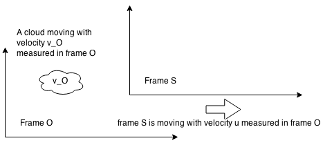
Fig. 20 Addition of velocities

Recall that in special relativity, velocity addition is

(10)\[v_S = \frac{u+v_O}{1+ \beta v/c},\]

where \(v_S\) is the velocity measured in moving frame S, \(v_O\) is the velocity measured in frame O. This \(\beta\) is the factor \(u/c\) where u is the velocity of the moving frame measure in frame O.

At the same time, we have the following hyper trig relation.

\[\tanh (\alpha + \beta) = \frac{\tanh \alpha + \tanh \beta}{1 + \tanh \alpha \tanh \beta}.\]

Isn’t this addition of angles the same as the velocity addition?

The algebra of relativity is mostly based on invariance of a new distance under a new rotation. Here we are not going to repeat the derivation of these transformations from the beginning, instead we would like to have a look at the really amazing part of this mathematical theory.

As shown in Fig. 20, we define quantities in two different frames, the frame O and frame S. The velocity of frame S measured in frame O is \(u\). Out of this velocity we define a quantity

\[\tanh \alpha_u = \frac{u}{c},\]

In fact, any velocity divided by speed of light should be a hyperbolic tangent,

\[\tanh \alpha_{v_x} = \frac{v_x}{c}.\]

With this definition of hyperbolic tangent, we notice that

\[\gamma = \frac{1}{\sqrt{1 - u^2/c^2}} = \cosh\alpha_u.\]

Suppose we have an object moving with velocity \(v_S\) in frame S. The velocity measured in frame O is the addition of the velocity of frame S itself and the velocity \(v_S\), except the addition rule is not the usual plus but the rule stated in Eq. ((10)). We apply the definitions of the hyperbolic trig function,

\[\frac{v_{S}}{c} = \tanh(\alpha_u + \alpha_{v_O}) = \frac{\tanh \alpha_{u} + \tanh \alpha_{v_0}}{1 + \tanh \alpha_{U} \tanh \alpha_{v_O}} = \frac{u/c + v_O/c}{1+ \frac{u}{c} \frac{v_{O}}{c}}.\]

We could imagine the algebra of velocities would be simply summations if we define ‘velocity’ as \(\arctan \frac{v_x}{c}\).

Addition of velocities is not that fundamental. What’s more important is the transformation of coordinate, as we have always been talking about. In the old school language, the coordinate transformation is

\[\begin{split}\begin{pmatrix} t_O\\ x_O \end{pmatrix} = \gamma \begin{pmatrix} 1 & u/c^2 \\ u & 1 \end{pmatrix}\begin{pmatrix} t_S\\ x_S \end{pmatrix},\end{split}\]

where

\[\gamma = \frac{1}{\sqrt{1 - u^2/c^2}} = \cosh\alpha_u.\]

If we use the language of hyperbolic trig functions, this transformation becomes

\[\begin{split}\begin{pmatrix} t_O\\ x_O \end{pmatrix} = &\cosh\alpha_u \begin{pmatrix} 1 & (\tanh \alpha_u)/c \\ c(\tanh\alpha_u) & 1 \end{pmatrix}\begin{pmatrix} t_S\\ x_S \end{pmatrix}\\ =& \begin{pmatrix} \cosh\alpha_u & (\sin \alpha_u)/c \\ c(\sin\alpha_u) & \cosh\alpha_u \end{pmatrix}\begin{pmatrix} t_S\\ x_S \end{pmatrix}.\end{split}\]

To make the transformation symmetric, we consider

\[\begin{split}\begin{pmatrix} c t_O\\ x_O \end{pmatrix} = \begin{pmatrix} \cosh\alpha_u & \sin \alpha_u \\ \sin\alpha_u & \cosh\alpha_u \end{pmatrix}\begin{pmatrix} ct_S\\ x_S \end{pmatrix}.\end{split}\]

Natural Unit

Look at these tedious steps. Why not just use natural units and set \(c=1\). We should.

This is basically the rotation matrix in hyperbolic spacetime.

Rotation in Euclidean Space

The rotations in Euclidean space is described as

\[\begin{split}\begin{pmatrix} x'\\ y' \end{pmatrix} = \begin{pmatrix} \cos\theta & -\sin \theta \\ \sin\theta & \cos\theta \end{pmatrix}\begin{pmatrix} x\\ y \end{pmatrix}.\end{split}\]

It is quite different from the rotations in Euclidean space.

Since we are talking about geometry, space-time diagram will be extremely important. The length contraction, time dilation, and even doppler shift can be explained and calculated using the hyperbolic trig functions. Triangles on the space-time diagram are described in Visualizations of Hyperbolic Space.

Time Dilation

Use a spacetime diagram.

Length Contraction

Use a spacetime diagram.

Footnotes

1. The Geometry of Special Relativity by Tevian Dray.

[1]	Actually, there are more general definations for Lapacian, which includes this d’Alembertian of course.

[2]	wiki:D’Alembert_operator

[Schutz2009]

(1, 2) A First Course in General Relativity